Repeated measures ANOVA in Python
April 2018
Welcome to this first tutorial on the Pingouin statistical package. In this tutorial, you will learn how to compute a two-way mixed design analysis of variance (ANOVA) using the Pingouin statistical package. This tutorial is mainly geared for beginner, and more advanced users can check the official Pingouin API.
Installation
To install Pingouin, you need to have Python 3 installed on your computer. If you are using a Mac or Windows, I strongly recommand installing Python via the
Anaconda distribution.
To install pingouin, just open a terminal and type the following lines:
pip install --upgrade pingouinOnce Pingouin is installed, you can simply load it in a python script, ipython console, or Jupyter notebook:
import pingouin as pgSimulate the data
For the sake of the example, let's say that we are interested in how meditation can improve school performances in primary school students. If we want to study that, one way would be to split a group of student into a
control group and a meditation group, i.e. a certain
number of students will be instructed to meditate for 20 minutes a day every day of the week, while the remaining students will be instructed not to change anything to their usual daily routine. This factor is our between-group factor.
Now, we want to examine how meditation significantly improves or worsens the performances over time, starting from the beginning of the school year (August) to the end of the school year. To study that, we are going to asses
their
school performances at three time points during the year: August (or time = 0 months), January (time = +6months) and June (time = +12 months).
To sum up, we have:
- A dependent variable: the test scores
- A within-group variable, time of the year, with three levels (August, January, June)
- A between-group variable, Group, with two levels (Control, Meditation)
- A subject variable, Subject
import pandas as pd
import numpy as np

# Let's assume that we have a balanced design with 30 students in each group
n = 30
months = ['August', 'January', 'June']

# Generate random data
np.random.seed(1234)
control = np.random.normal(5.5, size=len(months) * n)
meditation = np.r_[ np.random.normal(5.4, size=n),
                    np.random.normal(5.8, size=n),
                    np.random.normal(6.4, size=n) ]

# Create a dataframe
df = pd.DataFrame({'Scores': np.r_[control, meditation],
                   'Time': np.r_[np.repeat(months, n), np.repeat(months, n)],
                   'Group': np.repeat(['Control', 'Meditation'], len(months) * n),
                   'Subject': np.r_[np.tile(np.arange(n), 3),
                                    np.tile(np.arange(n, n + n), 3)]})
We can print the first lines of our dataframe using df.head():
| Group | Scores | Time | Subject |
|---|---|---|---|
| Control | 5.9714 | August | 0 |
| Control | 4.3090 | August | 1 |
| Control | 6.9327 | August | 2 |
| Control | 5.1873 | August | 3 |
| Control | 4.7794 | August | 4 |
Descriptive statistics
Now let's take a look at our data using the Seaborn package:
import seaborn as sns
sns.set()
sns.pointplot(data=df, x='Time', y='Scores', hue='Group', dodge=True, markers=['o', 's'],
	      capsize=.1, errwidth=1, palette='colorblind')
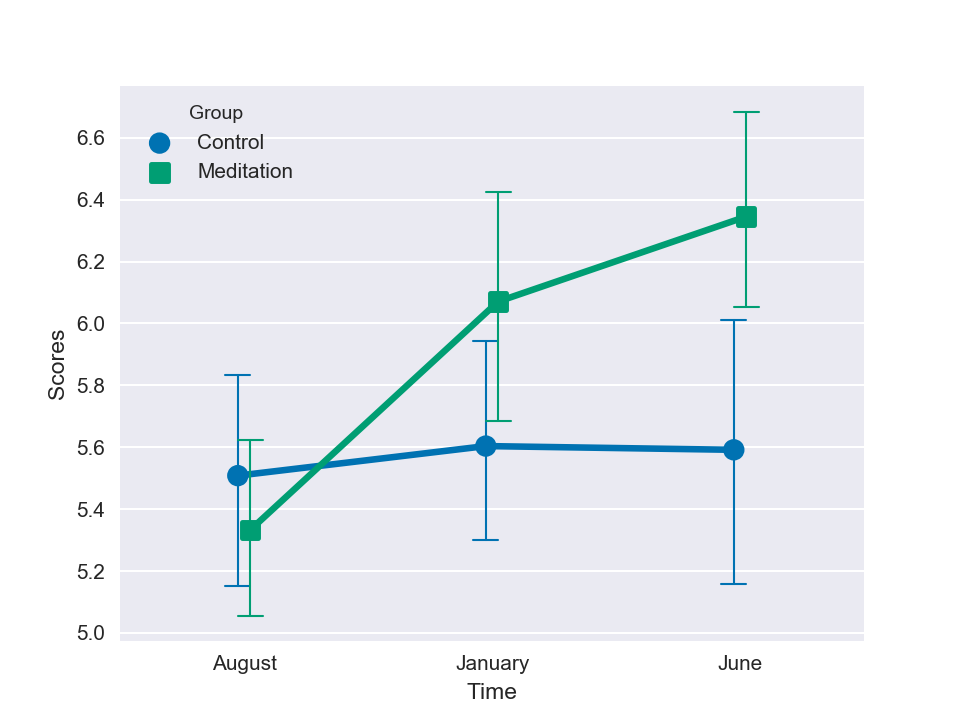
Visually, we can already see a clear improvement of the test scores over time in the meditators group. Let's look at the mean and standard deviations of the data:
df.groupby(['Time', 'Group'])['Scores'].agg(['mean', 'std']).round(2)| Time | Group | Mean | STD |
|---|---|---|---|
| August | Control | 5.51 | 1.03 |
| August | Meditation | 5.33 | 0.81 |
| January | Control | 5.60 | 0.90 |
| January | Meditation | 5.97 | 1.07 |
| June | Control | 5.59 | 1.18 |
| June | Meditation | 6.35 | 0.93 |
ANOVA
To test the significance of this effect, we will need to use a mixed-design ANOVA. That is where Pingouin comes into play. We are going to use the mixed_anova function with the following input arguments:
- dv: name of the column containing the dependant variables
- within: name of the column containing the within-group factor.
- between: name of the column containing the between-group factor.
- data: name of the pandas dataframe
import pingouin as pg
# Compute the two-way mixed-design ANOVA
aov = pg.mixed_anova(dv='Scores', within='Time', between='Group', subject='Subject', data=df)
# Pretty printing of ANOVA summary
pg.print_table(aov)
| Source | SS | DF1 | DF2 | MS | F | p-unc | np2 | eps |
|---|---|---|---|---|---|---|---|---|
| Group | 4.465 | 1 | 58 | 4.465 | 4.131 | 0.047 | 0.066 | - |
| Time | 9.359 | 2 | 116 | 4.679 | 4.940 | 0.008 | 0.078 | 0.998 |
| Interaction | 6.539 | 2 | 116 | 3.269 | 3.452 | 0.035 | 0.056 | - |
We can see that there is indeed a significant interaction, F(2, 116)=3.45, p=.035. The effect size (partial eta-square) of this interaction is .056.
However, this does not tell us which specific contrast is actually
significant.
For this reason, we need to perform post-hocs tests on the interaction. This can be done very easily using the pairwise_ttests
function:
posthocs = pg.pairwise_ttests(dv='Scores', within='Time', between='Group',
                              subject='Subject', data=df)
pg.print_table(posthocs)
which gives us (note that for display purpose I removed some rows and columns from the original table):
| Time | A | B | T-val | p-unc | Eff_size | Eff_type | BF10 |
|---|---|---|---|---|---|---|---|
| August | Control | Meditation | 0.733 | 0.466 | 0.187 | hedges | 0.329 |
| January | Control | Meditation | -1.434 | 0.157 | -0.365 | hedges | 0.619 |
| June | Control | Meditation | -2.744 | 0.008 | -0.699 | hedges | 5.593 |
Our visual impression is therefore confirmed: there is a significant increase in test scores in the meditator group 12 months after the beginning of the experiment (T=-2.7, p-unc=.008, Bayes Factor = 5.593). The corrected effect size (Hedges g) is approximately 0.70 and can therefore be considered, according to Cohen's rule of thumb, as large.
Appendix
Correction for multiple comparisons
If you have a large number of groups and/or measurements, you might want to correct the p-values for multiple comparisons. This can be done very easily using the padjust argument of the pairwise_ttests function:
pg.pairwise_ttests(dv='Scores', within='Time', between='Group', subject='Subject',
                   data=df, padjust='holm')
Missing values and unbalanced design
If one subject has one or more missing observations (for example, no tests scores in January), this subject will need to be removed from the ANOVA and post-hocs analyses. This is done automatically by the two aforementionned Pingouin functions. However, if your data really has a lot of missing values, you may want to consider alternative analyses methods, such as linear mixed-effects modelling, which better accomodates for missing data (see the excellent lme4 package in R).
On another note, Pingouin also works well with unbalanced design (i.e. different number of students per group). Please find an example in the full script of this tutorial (link above).
Other ANOVA functions in Pingouin
- pingouin.anova: One-way and two-way ANOVA
- pingouin.ancova: ANCOVA with one or more covariate(s)
- pingouin.welch_anova: One-way Welch ANOVA
- pingouin.rm_anova: One-way and two-way repeated measures ANOVA
- pingouin.mixed_anova: Mixed-design ANOVA
Further reading
- Lakens et al 2013: Calculating and reporting effect sizes to facilitate cumulative science: a practical primer for t-tests and ANOVAs.
- Altman et Krzywinski 2015: Points of Significance: Split plot design.