Correlation(s) in Python
July 2019
In this tutorial, you will learn how to calculate correlation between two or more variables in Python, using my very own Pingouin package.
Installation
To install Pingouin, you need to have Python 3 installed on your computer. If you are using a Mac or Windows, I strongly recommand installing Python via the
Anaconda distribution.
To install pingouin, just open a terminal and type the following lines:
pip install --upgrade pingouinOnce Pingouin is installed, you can simply load it in a python script, ipython console, or Jupyter lab:
import pingouin as pgCorrelation coefficient
The correlation coefficient (sometimes referred to as Pearson's correlation coefficient, Pearson's product-moment correlation, or simply r) measures the strength of the linear relationship between two variables. It is indisputably one of the most commonly used metrics in both science and industry. In science, it is typically used to test for a linear association between two dependent variables, or measurements.
In industry, specifically in a machine-learning context, it is used to discover collinearity between features, which may undermine the quality of a model.
The correlation coefficient is directly linked to the beta coefficient in a linear regression (= the slope of a best-fit line), but has the advantage of being standardized between -1 to 1 ; the former meaning a perfect negative linear relationship, and the latter a perfect positive linear relationship. In other words, no matter what are the original units of the two variables are, the correlation coefficient will always be in the range of -1 to 1, which makes it very easy to work with.
Finally, the correlation coefficient can be used to do hypothesis testing, in which case a so-called correlation test will return not only the correlation coefficient (the r value) but also the p-value, which, in short, quantifies the statistical significance of the test.
For more details on this, I recommend reading the excellent book “Statistical Thinking for the 21st Century” by Stanford's Professor Russ Poldrack.
Load the data
For the sake of the example, I generated a fake dataset that comprises the results of personality tests of 200 individuals, together with their age, height, weight and IQ. Please note that these data are randomly generated and not representative of real individuals.
The personality dimensions are defined according to the Big Five model (or OCEAN), and are typically measured on a 1 to 5 scale- Openness to experience (inventive/curious vs. consistent/cautious)
- Conscientiousness (efficient/organized vs. easy-going/careless)
- Extraversion (outgoing/energetic vs. solitary/reserved)
- Agreeableness (friendly/compassionate vs. challenging/detached)
- Neuroticism (sensitive/nervous vs. secure/confident)
import pandas as pd

df = pd.read_csv('data_corr.csv')
print('%i subjects and %i columns' % df.shape)
df.head()
| Age | IQ | Height | Weight | O | C | E | A | N |
|---|---|---|---|---|---|---|---|---|
| 56.0 | 110.0 | 158.0 | 57.1 | 3.9 | 3.5 | 4.2 | 4.0 | 2.5 |
| 46.0 | 85.0 | 168.7 | 74.1 | 4.0 | 3.2 | 3.2 | 3.4 | 2.6 |
| 32.0 | 94.0 | 162.8 | 74.1 | 3.4 | 3.5 | 2.9 | 2.8 | 2.8 |
| 60.0 | 95.0 | 166.5 | 77.9 | 3.5 | 2.8 | 3.6 | 3.2 | 2.9 |
| 25.0 | 112.0 | 164.9 | 75.5 | 4.0 | 2.9 | 3.3 | 3.2 | 3.0 |
Simple correlation between two columns
First, let's start by calculating the correlation between two columns of our dataframe. For instance, let's calculate the correlation between height and weight...Well, this is definitely not the most exciting research idea, but certainly one of the most intuitive to understand! For the sake of statistical testing, our hypothesis here will be that weight and height are indeed correlated. In other words, we expect that the taller someone is, the larger his/her weight is, and vice versa.
This can be done simply by calling the pingouin.corr function:
import pingouin as pg
pg.corr(x=df['Height'], y=df['Weight'])
| n | r | CI95% | r2 | adj_r2 | p-val | BF10 | power |
|---|---|---|---|---|---|---|---|
| 200 | 0.447 | [0.33 0.55] | 0.200 | 0.192 | 3.253278e-11 | 2.718e+08 | 1.000 |
Let's take a moment to analyze the output of this function:
- n is the sample size, i.e. how many observations were included in the calculation of the correlation coefficient
- r is the correlation coefficient, 0.45 in that case, which is quite high.
- CI95% are the 95% confidence intervals around the correlation coefficient
- r2 and adj_r2 are the r-squared and ajusted r-squared respectively. As its name implies, it is simply the squared r, which is a measure of the proportion of the variance in the first variable that is predictable from the second variable.
- p-val is the p-value of the test. The general rule is that you can reject the hypothesis that the two variables are not correlated if the p-value is below 0.05, which is the case. We can therefore say that there is a significant correlation between the two variables.
- BF10 is the Bayes Factor of the test, which also measure the statistical significance of the test. It directly measures the strength of evidence in favor of our initial hypothesis that weight and height are correlated. Since this value is very large, it indicates that there is very strong evidence that the two variables are indeed correlated. While they are conceptually different, the Bayes Factor and p-values will in practice often reach the same conclusion.
- power is the achieved power of the test, which is the likelihood that we will detect an effect when there is indeed an effect there to be detected. The higher this value is, the more robust our test is. In that case, a value of 1 means that we can be greatly confident in our ability to detect the significant effect.
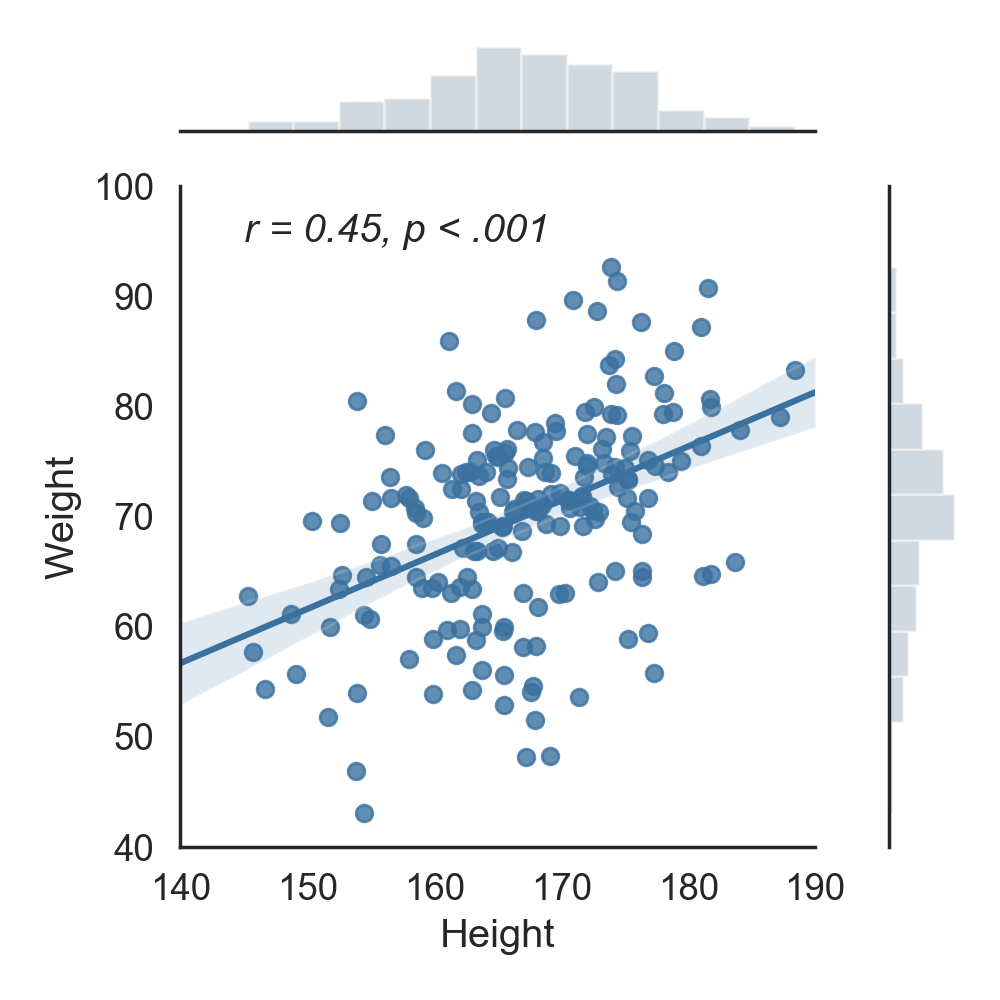
How does the correlation look visually? Let's plot this correlation using the Seaborn package:
import seaborn as sns
import matplotlib.pyplot as plt
from scipy.stats import pearsonr
sns.set(style='white', font_scale=1.2)

g = sns.JointGrid(data=df, x='Height', y='Weight', xlim=(140, 190), ylim=(40, 100), height=5)
g = g.plot_joint(sns.regplot, color="xkcd:muted blue")
g = g.plot_marginals(sns.distplot, kde=False, bins=12, color="xkcd:bluey grey")
g.ax_joint.text(145, 95, 'r = 0.45, p < .001', fontstyle='italic')
plt.tight_layout()
Pairwise correlation between several columns at once
What about the correlation between all the other columns in our dataframe? It would be a bit tedious to manually calculate the correlation between each pairs of columns in our dataframe (= pairwise correlation). Fortunately, Pingouin has a very convenient pairwise_corr function:
pg.pairwise_corr(df).sort_values(by=['p-unc'])[['X', 'Y', 'n', 'r', 'p-unc']].head()| X | Y | n | r | p-unc |
|---|---|---|---|---|
| Height | Weight | 200 | 0.447 | 0.000 |
| C | N | 200 | -0.368 | 0.000 |
| E | N | 200 | -0.344 | 0.000 |
| O | E | 200 | 0.273 | 0.000 |
| A | N | 200 | -0.174 | 0.014 |
For simplicity, we only display the the most important columns and the most significant correlation in descending order. This is done by sorting the output table on the p-value column (lowest p-value first) and using .head() to only display the first rows of the sorted table.
The pairwise_corr function is very flexible and has several optional arguments. To illustrate that, the code below shows how to calculate the non-parametric Spearman correlation coefficient (which is more robust to outliers in the data) on a subset of columns:
# Calculate the pairwise Spearman correlation
corr = pg.pairwise_corr(df, columns=['O', 'C', 'E', 'A', 'N'], method='spearman')
# Sort the correlation by p-values and display the first rows
corr.sort_values(by=['p-unc'])[['X', 'Y', 'n', 'r', 'p-unc']].head()| X | Y | n | r | p-unc |
|---|---|---|---|---|
| C | N | 200 | -0.344 | 0.000 |
| E | N | 200 | -0.316 | 0.000 |
| O | E | 200 | 0.240 | 0.001 |
| A | N | 200 | -0.184 | 0.009 |
| O | A | 200 | 0.066 | 0.353 |
One can also easily calculate a one-vs-all correlation, as illustrated in the code below.
# Calculate the Pearson correlation between IQ and the personality dimensions
corr = pg.pairwise_corr(df, columns=[['IQ'], ['O', 'C', 'E', 'A', 'N']], method='pearson')
corr.sort_values(by=['p-unc'])[['X', 'Y', 'n', 'r', 'p-unc']].head()| X | Y | r | p-unc |
|---|---|---|---|
| IQ | N | 0.126 | 0.075 |
| IQ | A | -0.083 | 0.241 |
| IQ | E | -0.056 | 0.430 |
| IQ | C | 0.013 | 0.855 |
| IQ | O | -0.006 | 0.934 |
There are many more facets to the pairwise_corr function, and this was just a short introduction. If you want to learn more, please refer to Pingouin's documentation and the example Jupyter notebook on Pingouin's GitHub page.
Correlation matrix
As the number of columns increase, it can become really hard to read and interpret the ouput of the pairwise_corr function. A better alternative is to calculate, and eventually plot, a correlation matrix. This can be done using Pandas and Seaborn:
df.corr().round(2)| Age | IQ | Height | Weight | O | C | E | A | N | |
|---|---|---|---|---|---|---|---|---|---|
| Age | 1.00 | -0.01 | -0.05 | -0.05 | -0.03 | -0.13 | -0.11 | -0.07 | 0.08 |
| IQ | -0.01 | 1.00 | 0.07 | 0.11 | -0.01 | 0.01 | -0.06 | -0.08 | 0.13 |
| Height | -0.05 | 0.07 | 1.00 | 0.45 | -0.12 | 0.03 | -0.07 | -0.03 | 0.07 |
| Weight | -0.05 | 0.11 | 0.45 | 1.00 | -0.11 | 0.10 | 0.00 | -0.00 | -0.15 |
| O | -0.03 | -0.01 | -0.12 | -0.11 | 1.00 | -0.02 | 0.27 | 0.07 | -0.04 |
| C | -0.13 | 0.01 | 0.03 | 0.10 | -0.02 | 1.00 | 0.01 | 0.07 | -0.37 |
| E | -0.11 | -0.06 | -0.07 | 0.00 | 0.27 | 0.01 | 1.00 | 0.02 | -0.34 |
| A | -0.07 | -0.08 | -0.03 | -0.00 | 0.07 | 0.07 | 0.02 | 1.00 | -0.17 |
| N | 0.08 | 0.13 | 0.07 | -0.15 | -0.04 | -0.37 | -0.34 | -0.17 | 1.00 |
corrs = df.corr()
mask = np.zeros_like(corrs)
mask[np.triu_indices_from(mask)] = True
sns.heatmap(corrs, cmap='Spectral_r', mask=mask, square=True, vmin=-.4, vmax=.4)
plt.title('Correlation matrix')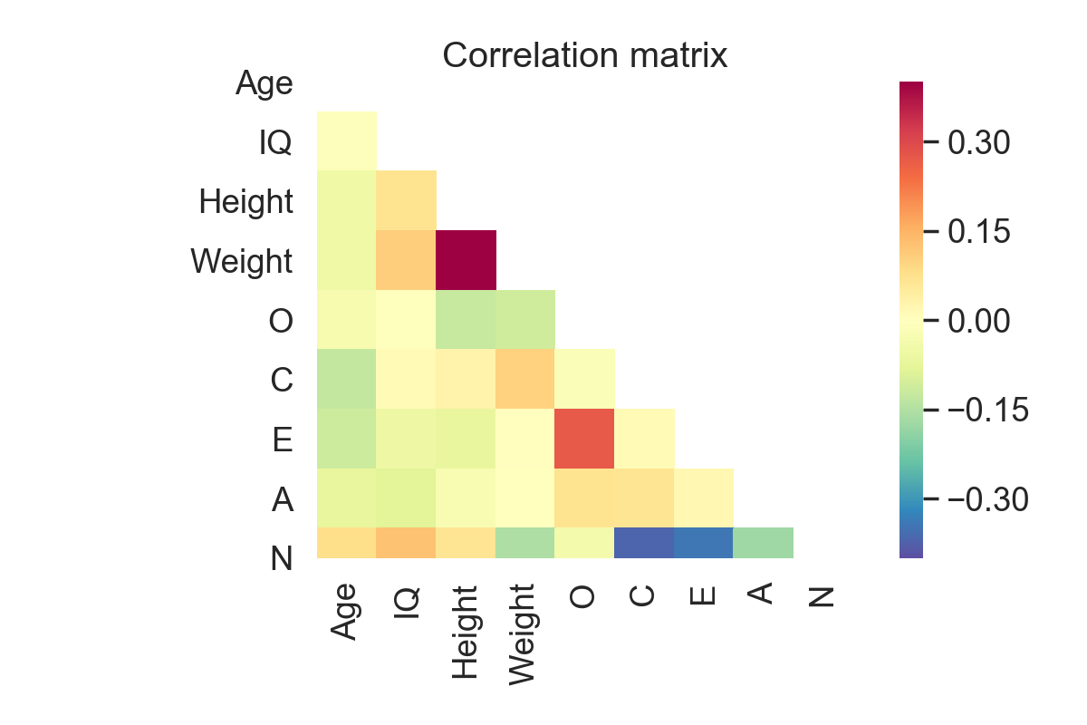
The only issue with these functions, however, is that they do not return the p-values, but only the correlation coefficients. Here again, Pingouin has a very convenient function that will show a similar correlation matrix with the r-value on the lower triangle and p-value on the upper triangle:
df.rcorr(stars=False)| Age | IQ | Height | Weight | O | C | E | A | N | |
|---|---|---|---|---|---|---|---|---|---|
| Age | - | 0.928 | 0.466 | 0.459 | 0.668 | 0.072 | 0.108 | 0.333 | 0.264 |
| IQ | -0.006 | - | 0.315 | 0.134 | 0.934 | 0.855 | 0.430 | 0.241 | 0.075 |
| Height | -0.052 | 0.071 | - | 0.000 | 0.081 | 0.646 | 0.316 | 0.696 | 0.351 |
| Weight | -0.053 | 0.106 | 0.447 | - | 0.117 | 0.15 | 0.986 | 0.977 | 0.029 |
| O | -0.031 | -0.006 | -0.123 | -0.111 | - | 0.793 | 0.000 | 0.319 | 0.575 |
| C | -0.128 | 0.013 | 0.033 | 0.102 | -0.019 | - | 0.839 | 0.355 | 0.000 |
| E | -0.114 | -0.056 | -0.071 | 0.001 | 0.273 | 0.014 | - | 0.776 | 0.000 |
| A | -0.069 | -0.083 | -0.028 | -0.002 | 0.071 | 0.066 | 0.02 | - | 0.014 |
| N | 0.079 | 0.126 | 0.066 | -0.154 | -0.04 | -0.368 | -0.344 | -0.174 | - |
Now focusing on a subset of columns, and highlighting the significant correlations with stars:
df[['O', 'C', 'E', 'A', 'N']].rcorr()| O | C | E | A | N | |
|---|---|---|---|---|---|
| O | - | *** | |||
| C | -0.019 | - | *** | ||
| E | 0.273 | 0.014 | - | *** | |
| A | 0.071 | 0.066 | 0.02 | - | * |
| N | -0.04 | -0.368 | -0.344 | -0.174 | - |