Raphael Vallat, PhD

CONN Toolbox

Plot denoised BOLD timeseries of 2 ROIs

February 2017

A simple script to plot the BOLD denoised time-series of two specified ROIs from CONN Toolbox ROI.mat file

• The full script can be downloaded on my GitHub repository

---

Define analysis info

• Info.wdir: path to your CONN/results/preprocessing folder which contains the denoised time-series of all the ROIs (see this post for a exhaustive review of CONN output files.


• Info.session: if you have several session (i.e. pre / post resting-state scans), enter the number of the desired session or put 0 for a temporal concatenation of all sessions.


• Info.nsub: number of subjects


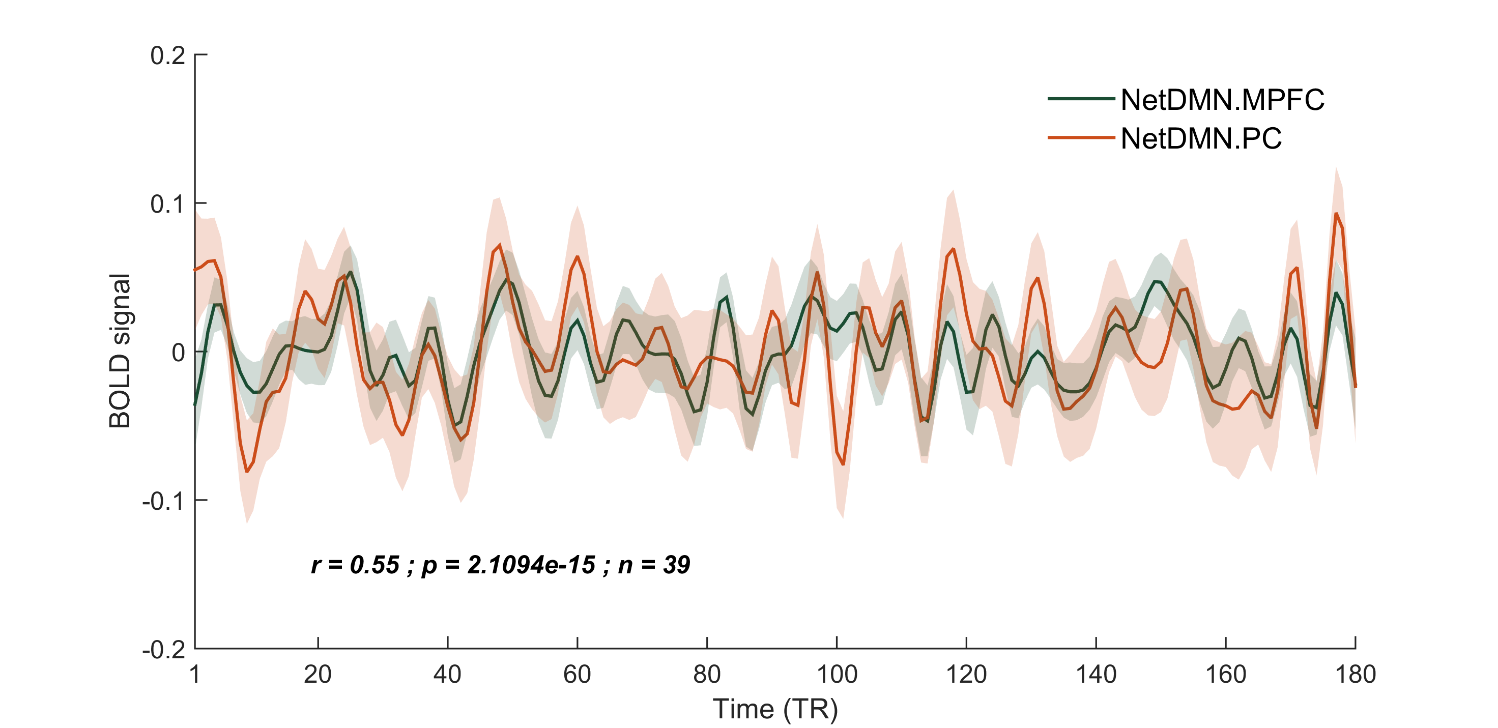
• ROI.ROIX_name: name of the ROIs you want to plot, as they appear in CONN Toolbox. In this example I am using two classic nodes of the default mode network, i.e. the medial prefrontal cortex and precuneous.



Info            = [];
Info.wdir       = 'C:/PhD/fMRI/CONN/conn_39s_preproc/results/preprocessing/';
Info.session    = 1;        % 0 for all sessions, 1=session1, 2=session2, etc...
Info.nsub       = 39;       % Total number of subjects

% ROI is the main structure containing ROI names, data
ROI             = [];
ROI.ROI1_data   = [];
ROI.ROI2_data   = [];

% Select pair of ROIs
ROI.ROI1_name   = 'NetDMN.MPFC';
ROI.ROI2_name   = 'NetDMN.PC';

% Define outpath and outfilename
Info.outdir     = pwd;
Info.outfile    = [ Info.outdir '/TS_' ROI.ROI1_name  '_' ROI.ROI2_name '_RUN'
			num2str(Info.session) '.png' ];

---

Import data

Once this is done, the next step is to load the ROI mat file of each subject and find the two time-series of interest

for i=1:Info.nsub

    % Loading .MAT file
    matfile = [ 'ROI_Subject0', num2str(i, '%02i') ,'_Condition000.mat' ];

    %fprintf('\nLoading:\t %s', matfile);

    load([Info.wdir matfile]);

    ROI.names   = names;
    ROI.dsess   = data_sessions;

    % Find index of selected ROIs
    ROI.ROI1_idx    = find(strcmp(ROI.ROI1_name, names));
    ROI.ROI2_idx    = find(strcmp(ROI.ROI2_name, names));

    % Extract BOLD data
    ROI.ROI1_data   = [ ROI.ROI1_data , cell2mat(data(ROI.ROI1_idx)) ];
    ROI.ROI2_data   = [ ROI.ROI2_data , cell2mat(data(ROI.ROI2_idx)) ];

    % Select sessions
    if Info.session == 0 ;
        ROI.cond = find(ROI.dsess);
    else
        ROI.cond = find(ROI.dsess == Info.session);
    end
end

---

Compute means, sem and correlations

Then compute the mean timeseries with its corresponding standard error of the mean as well as the correlation coefficient between the two mean time-series.

% Compute mean, std and sem
ROI.ROI1_mean   = mean(ROI.ROI1_data, 2);
ROI.ROI1_std    = std(ROI.ROI1_data, 0, 2);
ROI.ROI1_sem    = ROI.ROI1_std / sqrt(Info.nsub);

ROI.ROI2_mean   = mean(ROI.ROI2_data, 2);
ROI.ROI2_std    = std(ROI.ROI2_data, 0, 2);
ROI.ROI2_sem    = ROI.ROI2_std / sqrt(Info.nsub);

% Correlation between mean timeseries
[rho_mean, pval_mean] = corr(ROI.ROI1_mean(ROI.cond), ROI.ROI2_mean(ROI.cond));

By default CONN toolbox applies a Fisher transform to all the R correlation values in order to homogenize the variance. If you prefer to compute the Z fisher-transformed value of your correlation coefficient, simply use the atanh(r) function of Matlab.

---

Plot

Mean time-series

% Create plot variables
ROI.x       = [ 1:length(ROI.cond) ]';
ROI.ROI1_Y  = ROI.ROI1_mean(ROI.cond,:);
ROI.ROI2_Y  = ROI.ROI2_mean(ROI.cond,:);
ROI.ROI1_dy = ROI.ROI1_sem(ROI.cond, :);
ROI.ROI2_dy = ROI.ROI2_sem(ROI.cond, :);

set(0,'defaultfigurecolor',[ 1 1 1 ])
set(0,'DefaultAxesFontSize', 10)
fig = figure;
set(gcf,'Units','inches', 'Position',[0 0 6 3])
line_color = [ 0.1 0.3 0.2 ; 0.8 0.3 0.1 ];
set(gca, 'ColorOrder', line_color, 'NextPlot', 'replacechildren');

% Plot average ROI BOLD signal
plot(ROI.x, ROI.ROI1_Y, ROI.x, ROI.ROI2_Y, 'LineWidth', 1.5)
hold on
legend(ROI.ROI1_name, ROI.ROI2_name, 'Location', 'northeast')
legend('boxoff')

Semi-transparent continuous error bar

if Info.nsub > 1
    fill([ROI.x;flipud(ROI.x)],[ROI.ROI1_Y-ROI.ROI1_dy;flipud(ROI.ROI1_Y+ROI.ROI1_dy)],
				line_color(1,:),'linestyle','none', 'FaceAlpha', .2);
    fill([ROI.x;flipud(ROI.x)],[ROI.ROI2_Y-ROI.ROI2_dy;flipud(ROI.ROI2_Y+ROI.ROI2_dy)],
				line_color(2,:),'linestyle','none', 'FaceAlpha', .2);
end

Annotate the correlation value

dim = [.2 .2 .3 .1];
str = [ 'r = ', num2str(round(rho_mean, 2), '%.2f'), ' ; p = ',
			num2str(pval_mean), ' ; n = ', num2str(Info.nsub) ];
annotation('textbox',dim,'String',str,'FitBoxToText','on', 'EdgeColor',
			'none', 'FontWeight', 'bold', 'FontAngle', 'italic');

Set axis properties

y_lim = [ -0.2 0.2 ];
ylim(y_lim);
xlim([0 length(ROI.cond)]);
%set(gca, 'XColor', 'w');   % Mask x-axis
ylabel('BOLD signal');
xlabel('Time (TR)');
set(gca, 'XTick', [ 0:20:length(ROI.cond) ]);
grid off
box off

% Savefig 600 dpi
fig.PaperPositionMode = 'auto';
print(Info.outfile,'-dpng','-r600')

clearvars -except ROI Info

And that's it!